|
JKQTPlotter trunk/v5.0.0
an extensive Qt5+Qt6 Plotter framework (including a feature-richt plotter widget, a speed-optimized, but limited variant and a LaTeX equation renderer!), written fully in C/C++ and without external dependencies
|
|
JKQTPlotter trunk/v5.0.0
an extensive Qt5+Qt6 Plotter framework (including a feature-richt plotter widget, a speed-optimized, but limited variant and a LaTeX equation renderer!), written fully in C/C++ and without external dependencies
|
This tutorial project (see ./examples/datastore_statistics/) explains several advanced functions of JKQTPDatastore in combination with the [JKQTPlotter Statistics Library] conatined in JKQTPlotter.
Note that there are additional tutorial explaining other aspects of data mangement in JKQTPDatastore:
The source code of the main application can be found in datastore_regression.cpp. This tutorial cites only parts of this code to demonstrate different ways of performing regression analysis.
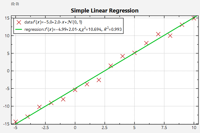
First we generate a set of datapoints (x,y), which scatter randomly around a linear function.
... and we visualize this data with a simple scatter graph:
Now we can caluate the regression line (i.e. the two regression coefficients a and b of the function f(x)=a+b*x) using the function jkqtpstatLinearRegression() from the [statisticslibrary]:
... and add a JKQTPXFunctionLineGraph to draw the resulting linear function:
These two steps can be simplified using an "adaptor":
... or even shorter:
Here the x- and y-columns from the JKQTPXYGraph-based graph graphD (see above) are used as datasources for the plot.
The plot resulting from any of the variants above looks like this:
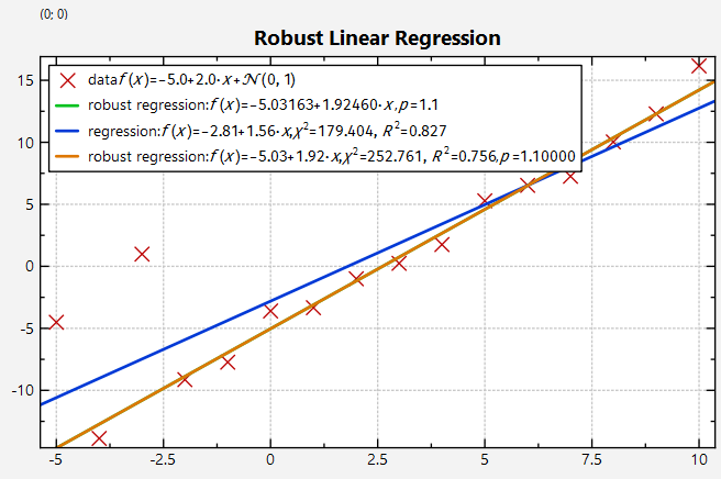
Sometimes data contains outliers that can render the results of a regression analysis inaccurate. For such cases the JKQTPlotter Statistics Library offers the function jkqtpstatRobustIRLSLinearRegression(), which is a drop-in replacement for jkqtpstatLinearRegression() and solves the optimization problem a) in the Lp-norm (which is more robust to outliers) and b) uses the iteratively reweighted least-squares algorithm (IRLS), which performs a series of regressions, where in each instance the data-points are weighted differently. The method assigns a lower weight to those points that are far from the current best-fit (typically the outliers) and thus slowly comes nearer to an estimate that is not distorted by the outliers.
To demonstrate this method, we use the same dataset as above, but add a few outliers:
Note the outliers ar x=-5 and x=-3!
With this dataset we can use the same code as above, but with jkqtpstatRobustIRLSLinearRegression() instead of jkqtpstatLinearRegression():
Also for the robust regression, there are two shortcuts in the form of "adaptors":
and
The following screenshot shows the result of the IRLS regression analysis and for comparison the normal linear regression for the same dataset (plotted using jkqtpstatAddLinearRegression(graphD);):
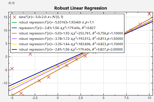
The following screenshot shows the influence of the regularization parameter p (default value 1.1) onto the fit result:
Another option to react to measurement errors is to take these into account when calculating the regression. To do so, you can use weighted regression that uses the measurement errors as inverse weights. This algorithm is implemented in the function jkqtpstatLinearWeightedRegression().
First we generate again a set of datapoints (x,y), which scatter randomly around a linear function. In addition we calculate an "error" err for each datapoint:
We use distribution de to draw deviations from the ideal linear function from the range 0.5...1.5. then - for good measure - we use a second distribution ddecide (dice tossing) to select a few datapoints to have a 4-fold increased error.
Finally we visualize this data with a simple scatter graph with error indicators:
Now we can caluate the regression line (i.e. the two regression coefficients a and b of the function f(x)=a+b*x) using the function jkqtpstatLinearWeightedRegression() from the [statisticslibrary]:
Note that in addition to the three data-columns we also provided a C++ functor jkqtp_inversePropSaveDefault(), which calculates 1/error. This is done, because the function jkqtpstatLinearWeightedRegression() uses the data from the range datastore1->begin(colWLinE) ... datastore1->end(colWLinE) directly as weights, but we calculated errors, which are inversely proportional to the weight of each data point when solving the least squares problem, as data points with larger errors should be weighted less than thos with smaller errors (outliers).
Again these two steps can be simplified using an "adaptor":
... or even shorter:
Here the x- and y-columns from the JKQTPXYGraph-based graph graphE (see above) and the weights from the error column of graphE are used as datasources for the plot. This function implicitly uses the function jkqtp_inversePropSaveDefault() to convert plot errors to weights, as it is already clear that we are dealing with errors rather than direct weights.
The plot resulting from any of the variants above looks like this:
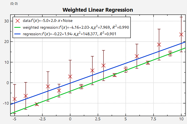
For this plot we also added a call to
which performs a simple non-weighted regression. The difference between the two resulting linear functions (blue: simple regression, green: weighted regression) demonstrates the influence of the weighting.
In addition to the simple linear regression model f(x)=a+b*x, it is also possible to fit a few non-linear models by transforming the data:
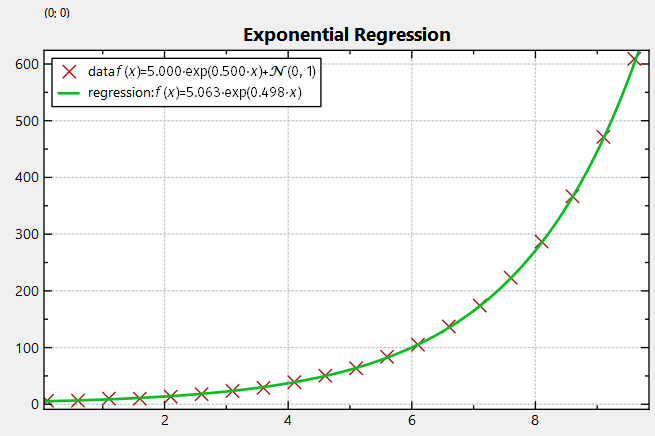
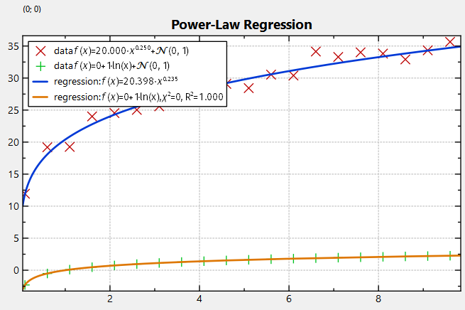
To demonstrate these fitting options, we first generate data from an exponential and a power-law model. Note that we also add normally distributed errors, but in order to ensure that we do not obtain y-values <0, we use loops that draw normally distributed random numbers, until this condition is met:
The generated data is visualized with scatter-plots:
Now we can fit the regression models using jkqtpstatRegression(), which receives the model type as first parameter:
The regression models can be plotted using a JKQTPXFunctionLineGraph. the fucntion to plot is again generated by calling jkqtpStatGenerateRegressionModel(), but now with the parameters determined above the respective lines. Note that jkqtpstatRegressionModel2Latex() outputs the model as LaTeX string, which can be used as plot label.
The resulting plot looks like this:
Of course also "adaptors" exist that allow to perform the steps above in a single function call:
... or even shorter:
Also note that we used the function jkqtpstatRegression() above, which performs a linear regression (internally uses jkqtpstatLinearRegression()). But there also exist variants for robust IRLS regression adn weighted regression:
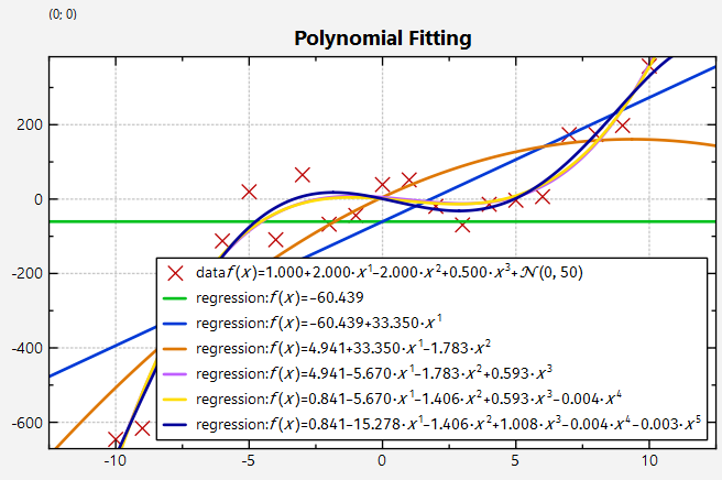
Finally the JKQTPlotter Statistics Library also supports one option for non-linear model fitting, namely fitting of polynomial models. This is implemented in the function jkqtpstatPolyFit().
To demonstrate this function we first generate data from a poylnomial model (with gaussian noise):
The function jkqtp_polyEval() is used to evaluate a given polynomial (coefficients in pPoly) at a position x.
The generated data is visualized with scatter-plots:
Here the function jkqtp_polynomialModel2Latex() generates a string from a polynomial model.
Now we can call jkqtpstatPolyFit() to fit different polynomial regression models to the data:
Each model is also ploted using a JKQTPXFunctionLineGraph. The plot function assigned to these JKQTPXFunctionLineGraph is generated by calling jkqtp_generatePolynomialModel(), which returns a C++-functor for a polynomial.
The resulting plots look like this (without added gaussian noise):
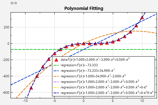
... and with added gaussian noise:
Of course also the "adaptor" shortcuts are available:
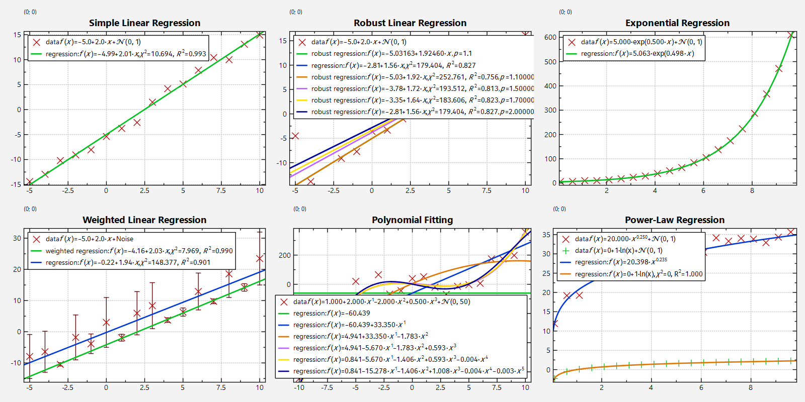
The output of the full test program datastore_regression.cpp looks like this: