|
JKQTPlotter trunk/v5.0.0
an extensive Qt5+Qt6 Plotter framework (including a feature-richt plotter widget, a speed-optimized, but limited variant and a LaTeX equation renderer!), written fully in C/C++ and without external dependencies
|
|
JKQTPlotter trunk/v5.0.0
an extensive Qt5+Qt6 Plotter framework (including a feature-richt plotter widget, a speed-optimized, but limited variant and a LaTeX equation renderer!), written fully in C/C++ and without external dependencies
|
Classes derived from JKQTPCoordinateAxis implements all the functionality needed for a coordinate axis:
Most of the actual draw and measure functions have to be implemented in descendents of this class (namely JKQTPHorizontalAxis and JKQTPVerticalAxis, as they are specific to whether the axis is drawn horizontally or vertically.
Each axis is split up into several parts, as depicted in this image:
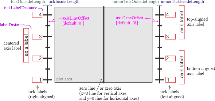
Which parts to actually draw is set by the diverse properties.
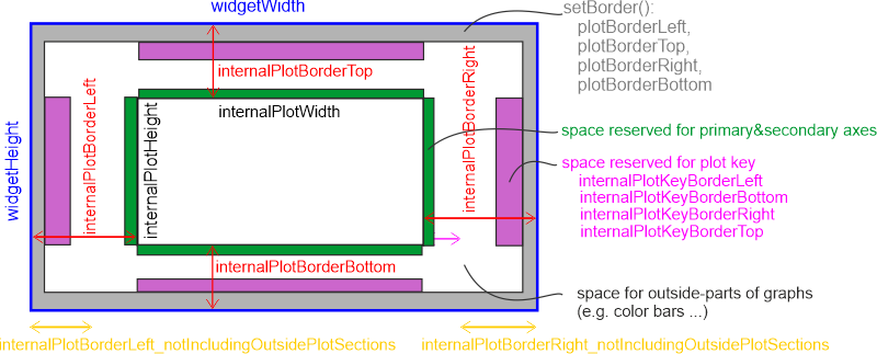
The plot itself is positioned inside the widget (see Plot Sizes & Borders for details). You simply supply the widget dimensions and the border widths between the plot and the widget. The Object then calculates the size of the plot:
The plot shows the parameter range xmin ... xmax and ymin ... ymax. Note that if you plot logarithmic plots you may only plot positive (>0) values. Any other value may lead to an error or unpredictable behaviour.
From these parameters the object calculates the scaling laws for plotting pints to the screen. The next paragraphs show all calculations for x- and y-coordinates, ahough this class only implements a generic form. The actual calculation is also influenced by the parameters set in the child classes!
These parameters are common to all scaling laws. The next image explains these formulas:
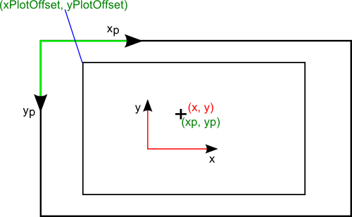
The actual scaling laws 
![\[ x_p(\mbox{xmin})=\mbox{xPlotOffset},\ \ \ \ \ x_p(\mbox{xmax})=\mbox{xPlotOffset}+\mbox{plotWidth} \]](form_221_dark.png)
![\[ y_p(\mbox{ymax})=\mbox{yPlotOffset},\ \ \ \ \ y_p(\mbox{ymin})=\mbox{yPlotOffset}+\mbox{plotHeight} \]](form_222_dark.png)
Here 

If you assume a linear scaling law.
![\[ x_p(x)=\mbox{xoffset}+x\cdot\mbox{xscale} \ \ \ \ \ \ \ \ \ y_p(y)=\mbox{yoffset}-y\cdot\mbox{yscale} \]](form_224_dark.png)
you can derive:
![\[ \mbox{xscale}=\frac{\mbox{plotWidth}}{\mbox{xwidth}},\ \ \ \ \ \ \mbox{xoffset}=\mbox{xPlotOffset}-\mbox{xmin}\cdot\mbox{xscale} \]](form_225_dark.png)
![\[ \mbox{yscale}=\frac{\mbox{plotHeight}}{\mbox{ywidth}},\ \ \ \ \ \ \mbox{yoffset}=\mbox{yPlotOffset}+\mbox{ymax}\cdot\mbox{yscale} \]](form_226_dark.png)
If you have a logarithmic axis (i.e. we plot 


![\[ x_p(x)=\mbox{xoffset}+\frac{\log(x)}{\log(\mbox{logXAxisBase})}\cdot\mbox{xscale} \ \ \ \ \ \ \ \ \ y_p(y)=\mbox{yoffset}-\frac{\log(y)}{\log(\mbox{logYAxisBase})}\cdot\mbox{yscale} \]](form_229_dark.png)
From these we can calculate their parameters with the same defining equations as above:
![\[ \mbox{xscale}=\frac{\mbox{plotWidth}\cdot\log(\mbox{logXAxisBase})}{\log(\mbox{xmax})-\log(\mbox{xmin})},\ \ \ \ \ \ \mbox{xoffset}=\mbox{xPlotOffset}-\frac{\log(\mbox{xmin})}{\log(\mbox{logXAxisBase})}\cdot\mbox{xscale} \]](form_230_dark.png)
![\[ \mbox{yscale}=\frac{\mbox{plotHeight}\cdot\log(\mbox{logYAxisBase})}{\log(\mbox{ymax})-\log(\mbox{ymin})},\ \ \ \ \ \ \mbox{yoffset}=\mbox{yPlotOffset}+\frac{\log(\mbox{ymax})}{\log(\mbox{logYAxisBase})}\cdot\mbox{yscale} \]](form_231_dark.png)
The object implements the above coordinate transformations in the (inline) method x2p(). The inverse transformations are implemented in p2x(). They can be used to show the system coordinates of the current mouse position.
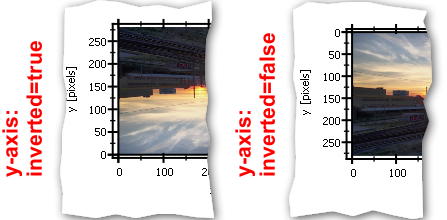
In some cases it may be necessary to invert the direction of increasing coordinates on an axis. One such case is image analysis, as computer images usually have coordinates starting with (0,0) at the top left and increasing to the right (x) and down (y). You can invert any axis by setting setInverted(true).
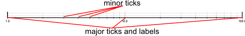
This section explains how this component draws the ticks on coordinate axes and the grids that may be drawn below the plots. In principle both - grids and axes - are drawn the same way, i.e. with the same step widths. There are two types of ticks and grids: The major and the minor ticks/grids. The major ticks also show a label that denotes the value they represent. Between two major ticks the axis shows JKQTPCoordinateAxisStyle::minorTicks small ticks that are not accompanied by a label. The next image shows an example of an axis:
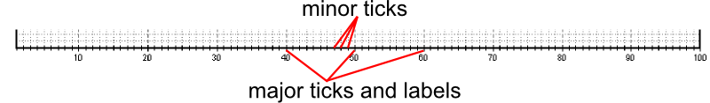
For the labels this class also uses an algorithm that extimates the number of valid digits (after the comma) that are needed so that two adjacent labels do not show the same text, so if you plot the range 1.10 .. 1.15 The algorithm will show at least two valid digits, as with one digit the labels would be 1.1, 1.1, 1.1, 1.1, 1.1, 1.1. With two digits they are 1.10, 1.11, 1.12, 1.13, 1.14, 1.15. The class may also use a method that can write 1m instead of 0.001 and 1k instead of 1000 (the algorithm supports the "exponent letters" f, p, n, u, m, k, M, G, T, P. The latter option may (de)activated by using showXExponentCharacter and showYExponentCharacter.
For grids applies the same. There are two grids that are drawn in different styles (often the major grid is drawn thicker and darker than the minor grid).
The minor ticks and grid lines are generated automatically, depending in the setting of JKQTPCoordinateAxisStyle::minorTicks. These properties give the number of minor ticks between two major ticks, so if the major ticks are at 1,2,3,... and you want minor ticks at 1.1, 1.2, 1.3,... then you will have to set JKQTPCoordinateAxisStyle::minorTicks=9 as there are nine ticks between two major ticks. So the minor tick spacing is calculated as:
![\[ \Delta\mbox{MinorTicks}=\frac{\Delta\mbox{ticks}}{\mbox{minorTicks}+1} \]](form_232_dark.png)
The same applies for logarithmic axes. If the major ticks are at 1,10,100,... and you set JKQTPCoordinateAxisStyle::minorTicks=9 the program will generate 9 equally spaced minor ticks in between, so you have minor ticks at 2,3,4,...,11,12,13,... This results in a standard logarithmic axis. If you set JKQTPCoordinateAxisStyle::minorTicks=1 then you will get minor ticks at 5,15,150,...
The major tick-tick distances of linear axes may be calculated automatically in a way that the axis shows at least a given number of ticks JKQTPCoordinateAxisStyle::minTicks. The algorithm takes that tick spacing that will give a number of ticks per axis nearest but ">=" to the given JKQTPCoordinateAxisStyle::minTicks. The Algorithm is described in detail with the function calcLinearTickSpacing(). To activate this automatic tick spacing you have to set autoAxisSpacing=true.
In some cases it is desired to put the axis ticks not at 1,2,3,... but rather at 


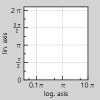
You can use these methods to set such a factor: